This page gives a short description of the complete GUI, sorted by menu item. For a more detailed description, see the corresponding wiki pages. There you will find more explanations and references.
¶ Menu
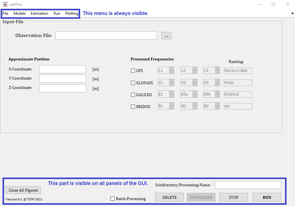
¶ File
Set Input File: Select a GNSS observation file in RINEX version 2+, the GNSS, and the frequencies to be processed. The observation ranking defines which observation type is preferred for each GNSS. Characters on the left have a higher order and are preferred. The approximate position values are automatically taken from the RINEX observation file header. You can enter [0,0,0] if no approximate is known.
Batch Processing: This panel allows you to process multiple observation files using the current GUI settings. Please not that you have to activate 'Batch-Processing' checkbox at the bottom of the GUI for batch processing.
Parameter Files: Save or load the parameters to/from the GUI, which are all settings that are independent of the observation file. By loading the parameters from another processing, you can process the currently selected observation file with identical settings. For example, loading the default parameters will reset the GUI settings to the default values and keep the current observation file.
Settings Files: Save or load all settings from/to the GUI. By loading a settings file, you can reprocess with entirely the same settings.
Exit: Close the GUI
Jump to Table of Content
¶ Models
Orbit/Clock: This panel allows you to select the orbit and clock products to be used for the PPP solution. You can either select precise products from an analysis centre and define the solution (e.g. final, rapid or MGEX), or use the broadcast navigation message alongside an optional correction stream. Alternatively, you can manually select orbit and clock files.
Biases: This panel defines the satellite biases that will be used. These biases are essential for the PPP solution, particularly if you wish to perform PPP-AR.
Ionosphere: This is a critical panel because it which PPP model is used and defines how the ionosphere is considered. The main options are as follows: The conventional PPP approach uses the two-frequency, ionosphere-free linear combination (IFLC). You can also use the uncombined PPP model ('Estimate'), optionally applying an ionospheric constraint ('Estimate with ... as constraint'). Furthermore, the decoupled clock model is available ('Estimate, decoupled clock').
Troposphere: This panel defines how the troposphere is treated. You can choose between different models and enable estimation of the remaining residual zenith wet delay (ZWD).
Other corrections: In this panel, you can enable or disable different error sources for modelling purposes. The cycle-slip detection settings can also be found here.
Kinematic: Essential settings for kinematic data processing can be configured on this panel.
Jump to Table of Content
¶ Estimation
Ambiguity Fixing: From this panel, you can enable PPP with Ambiguity Resolution (PPP-AR) and configure various settings for the fixed solution. Make sure that you have defined suitable satellite (phase) biases for PPP-AR.
Adjustment: This panel is used to define the parameter estimation (e.g., Kalman filter or no filter). The stochastic model is defined here.
Weighting: On this panel you can define the stochastics of the observations and their weighting (e.g., depending on GNSS or frequency).
¶ Run
Processing options: This panel contains several basic and essential processing settings. Most importantly, the processing method defines which measurements (code, phase, Doppler) will be processed and the time span of the observation file to be processed. You can also specify the resets of the PPP solution, which allows you to study the convergence behavior in more detail.
Export options: In this panel you can enable/disable various output files. Furthermore, you can decide which variables raPPPid will save after processing.
Jump to Table of Content
¶ Plotting
Single Plot: With this panel, you can open plots of the processing of a single observation file. Please note that it is also possible to stack the results of multiple processings defined by the Multi-Plot Table and create these for all of them ('Use Multi-Plot-Table') .
Multi Plot: This panel allows you to select the results of multiple processed observation files. They are then stored in the Multi-Plot Table. You can create different plots and statistics for them, focusing on the coordinate convergence behavior.
Jump to Table of Content
¶ Bottom part
Close All Figures: After confirmation, all other figures (e.g., plots, info-windows) except the GUI will be closed.
Batch-Processing: Enable this checkbox to start batch processing when hitting the "RUN" button. Please check the corresponding panel of the GUI. If this checkbox is disabled, the processing is started for a single file.
Subdirectory/Processing-Name: Here, you define the (sub)folder(s) where the processing is saved. If you leave this empty, a folder with the name of the RINEX file will be created in RESULTS. In this folder, a subfolder with "noname" and the date of the processing will be created. The chars of the processed GNSS are added automatically. Two examples of how you can use this, including pseudo-code (check replacePseudoCode.m for details):
RINEX file: EXAM000.00o, GPS and Glonass are processed, Subdirectory/Processing-Name: test → RESULTS/EXAM000_date/GR-test
RINEX file: EXAM000.00o, GPS and Glonass are processed, Subdirectory/Processing-Name: thisisatest/$stat/helloworld → RESULTS/GR-thisisatest/EXAM/EXAM000_date/helloworld
RESULTS: Opens the results folder of the last processing.
DELETE: Deletes the last processing. Additionally, you can delete the *.mat-files, which were produced from input files (e.g., SINEX bias file or clock file) to make the read-in faster. This might be useful if some error occurred.
DOWNLOAD: Download all input data that is currently required (GUI settings). Additionally, the processing settings are checked for validity. If the Batch Processing checkbox is selected, the data for the entire batch processing table is downloaded. This option ensures that missing input data will not cause errors. Therefore, it is recommended to use this option before processing, for example, when batch processing with a parfor loop.
STOP: Stop the current single file processing or the creation of plots.
RUN: Start the single-file or batch processing.
Jump to Table of Content