¶ Data
- Google Smartphone Decimeter Challenge 2021
- Google Smartphone Decimeter Challenge 2022
- EUSPA GNSS Raw Measurements Task Force
- Use a RINEX Logger Application (e.g., Google GnssLogger App plus UofC csv2rinex, Geo++ RINEX Logger, or rinex ON) to log your own RINEX data.
- However, raPPPid supports the raw sensor data logged with the Google GnssLogger App (since v2.0)
¶ Preparations
For optimal experience, consider the following (e.g., add information to the RINEX header):
- MARKER NAME: If you had placed the smartphone on a geodetic reference point, put the name here. Additionally, enter the known reference coordinates into raPPPid\DATA\COORDS\Coords.txt. Then, you can load these coordinates for plotting. Example line:
XXXX MARKER NAME - REC # / TYPE / VERS: Consider adding the smartphone's type (e.g., for creating a sensible processing name). Example line:
unknown HuaweiNova5T YAL-L21 REC # / TYPE / VERS - The header of RINEX files must include the record TIME OF FIRST OBS. However, some Android applications logging RINEX files do not write this line. In such a case, raPPPid reads the observation start date from the time-stamp of the first observation epoch. Alternatively, you can manually add this record to the header. Example line (year, day, month, hour, minute, second):
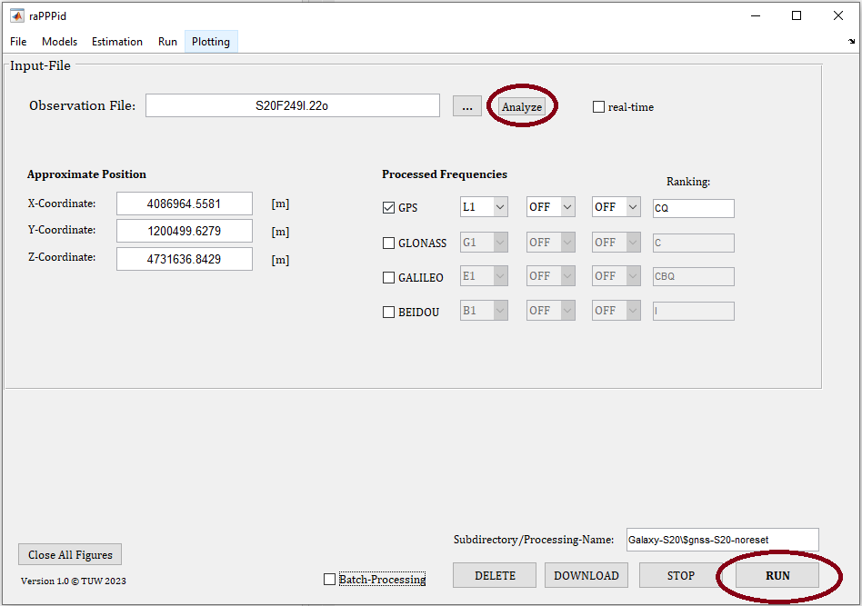
2021 5 25 8 44 39.0000195 GPS TIME OF FIRST OBS - The RINEX header of RINEX files recorded with smartphones might include GNSS or frequencies that were not observed. Consider using the Analyze button on the panel ‘Set Input-File’ and checking the created plots.
Experience showed that the following considerations and processing settings might improve the results:
- Make sure that duty cycling is deactivated.
- Check the exemplary parameter files suitable for smartphones.
- Disable the estimation of the ZWD. Complete modeling of the tropospheric delay might be sufficient depending on the smartphone device. However, for more extended time periods, estimating the ZWD might be necessary. Typically, this processing setting affects the height component the most, and you should play around with this option.
- A specific GNSS might introduce a considerable bias in the coordinates (e.g., all other GNSS that GPS in the provided Example Data).
- The Multipath Detection settings must be adapted to the specific smartphone device (e.g., thresholds).
- SNR weighting is recommended. However, it is difficult to recommend an SNR weighting function. Usually, this is a safe choice:
10.^-(max([55-snr,0]) ./ a). A meaningful choice of the coefficient a is 20 to 5 and depends on the specific smartphone (e.g., Samsung Galaxy = 20). - Consider the inconsistencies between the code, phase, and Doppler observations introduced by some applications used for logging RINEX files [Zangenehnejad et al., 2023]. Using Google GnssLogger App and the UofC csv2rinex tool is recommended for processing the raw sensor data output from the Google GnssLogger App. However, since version 2.0 raPPPid also accepts the raw GNSS measurement from Android smartphones recorded with the Google GnssLogger.
Jump to Table of Content
¶ Example 1: Code only
Download the example data as an archive. This archive contains a RINEX file (Samsung Galaxy S20 FE), an IONEX file (GIOMO predicted, an ionosphere model from TU Wien), and a settings file (settings.mat) as a starting point. Additionally, the archive contains the archived stream corrections for CNES as a backup. With this dataset, you should achieve similar results to the ones described in the raPPPid software paper.
Download raPPPid from GitHub and follow the instructions provided in the README.
Open Matlab and navigate to the WORK folder of raPPPid. Start the GUI with
raPPPid()Download and extract the input data mentioned above. Copy the RINEX and IONEX to the raPPPid folder structure with CopyData2Folders()
Load the downloaded settings.mat file to the GUI. Your GUI should look similar to the screenshot below. Consider testing the ‘Analyze’ button, which analyzes the RINEX files. This option prints information to the command window and creates some plots some plots only based on the data in the RINEX file.
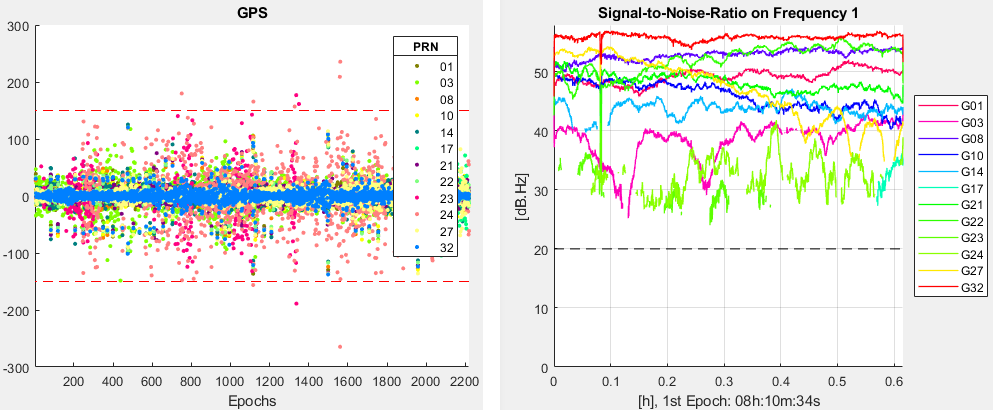
Start the processing with the RUN button. Be patient: The download and read-in of the input data will take some time (e.g., minutes) due to the characteristics of the stream corrections in the first processing. However, raPPPid will save the data in an internal format (*.mat). Therefore, the processing time is reduced massively in the further processings of this file.
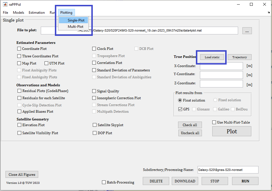
After the processing is finished, change to the panel Single-Plot. Load the true coordinates by hitting the button ‘Load static’ (the smartphone was placed on a geodetic reference point).
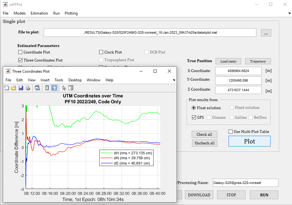
Select the ‘Three coordinates Plot’ and hit ‘Plot’. A figure should open. Change the limits of the x-axis by typing the following command into the command window: ylim([-3 3]). Congratulations! You have successfully processed and plotted raw GNSS data from a smartphone with raPPPid. Since the height component is worse than expected, you should do a re-processing: Activate the estimation of the ZWD and compare the results of these two processings and the ones included in the raPPPid paper.
Jump to Table of Content
¶ Example 2: Code + Phase
Since version 2.0, raPPPid can process the raw sensor data from Android smartphones logged with GnssLogger App from Google. By doing so, we have more control over the observations and avoid imperfections introduced by the RINEX logger (e.g., Zangenehnejad et. al, 2023), allowing, for example, the processing of the phase observation.
Download this example dataset, containing …
- raw sensor data collected with the GnssLogger App from Google and a Google Pixel 7 Pro on a geodetic reference point (PF04) on the rooftop of TU Wien
- an IONEX file (GIOMO predicted, an ionosphere model from TU Wien).
- the real-time correction data (SSRA00EUH00940.23C) of the Galileo High Accuracy Service (HAS), which was recorded with BKG Ntrip Client on the corresponding day and will be used in the second part of this example.
Use CopyData2Folders() to copy these files into the folder structure of raPPPid.
¶ GREC processing with CNES corrections

- Load the observation file (gnss_log_2023_04_04_10_26_54.txt, now contained in folder 2023/094).
- Deactivate the Galileo E5a frequency and deactivate QZSS.
- Furthermore, defining a sensible processing name is recommended.
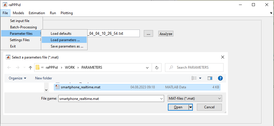
Load the parameter-file “smartphone_realtime.mat” into the GUI. Please change the following settings:
- On the panel Troposphere (Models, Troposphere, "Estimate ZWD from minute: 0"), activate the estimation of the Zenith Wet Delay.
- On the panel Processing-Options (Run, Processing Options) …
- change to “Code + and Phase” processing.
- activate “Adjust phase to code”.
- define the processing time span from epoch 1 to 1800.
- add a reset every 6 minutes.
- On the panel Other Corrections (Models, Other Corrections, Doppler-Shift), enable cycle slip detection with Doppler and set the threshold to 0.7 cycles.
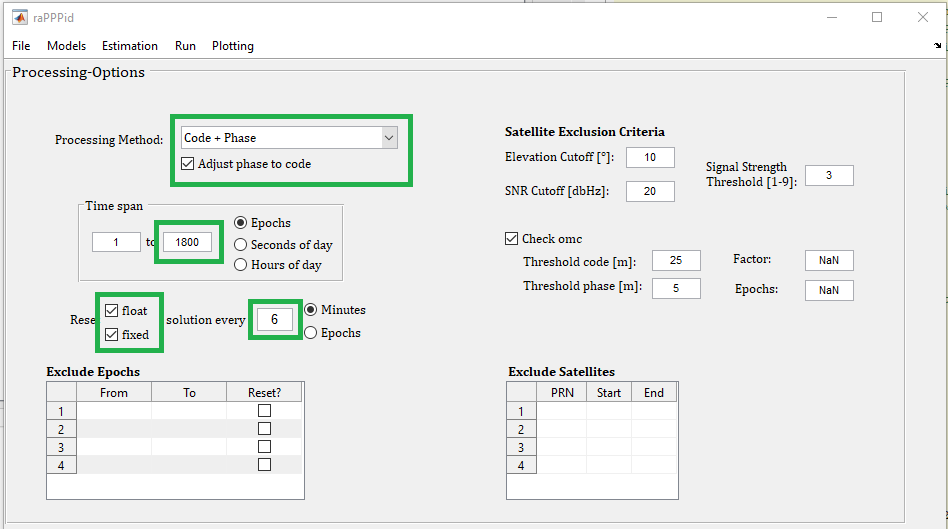
Now you can hit the RUN button. Please note that the first processing will take a considerable amount of time (e.g., 4-5 minutes) because the applied real-time corrections from the CNES archive are read-in.
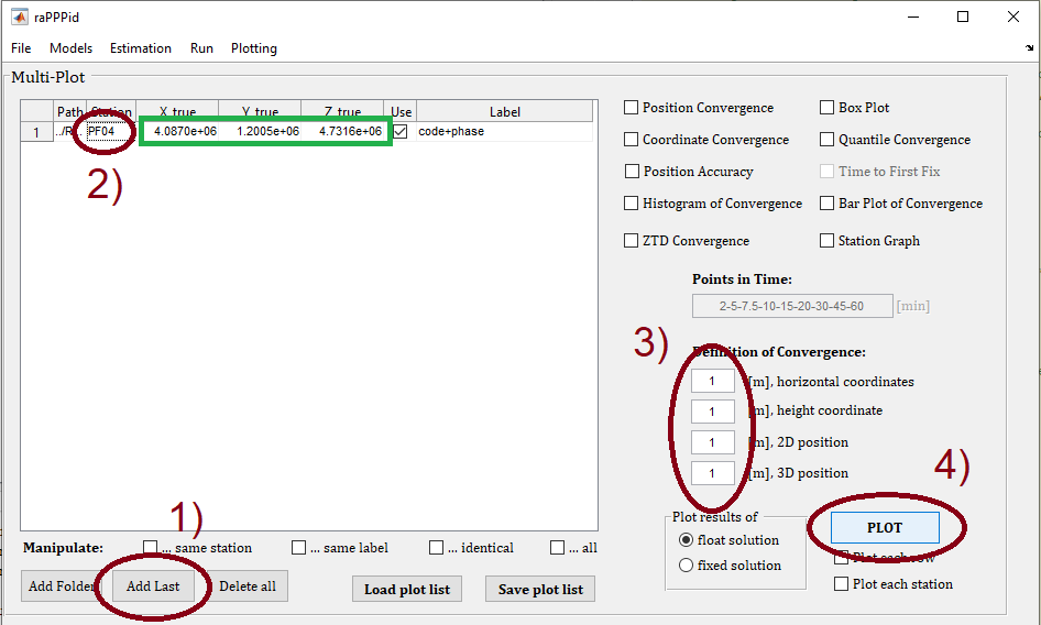
After the processing is finished, change to the panel Multi-Plot (under Plotting). Add the last processing ('Add last'). Load the reference coordinates by writing PF04 into the correct field and change the definition of convergence. Your Position Convergence plot should look similar to the following one.
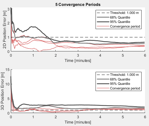
Congratulations! You have successfully processed raw GNSS data from a smartphone (code AND phase) and broken the one-meter accuracy level. If not, check if you really have activated the estimation of the ZWD. Thereby, you used real-time settings and corrections from CNES. In the next part of this example, the corrections from the Galileo HAS are used.
¶ GE processing with the Galileo HAS
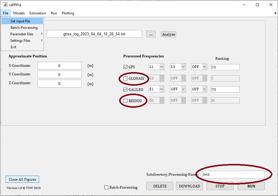
Change to the panel ‘Input File’ and deactivate GLONASS and BeiDou because the Galileo HAS provides corrections only for GPS and Galileo. Furthermore, define a sensible processing name.
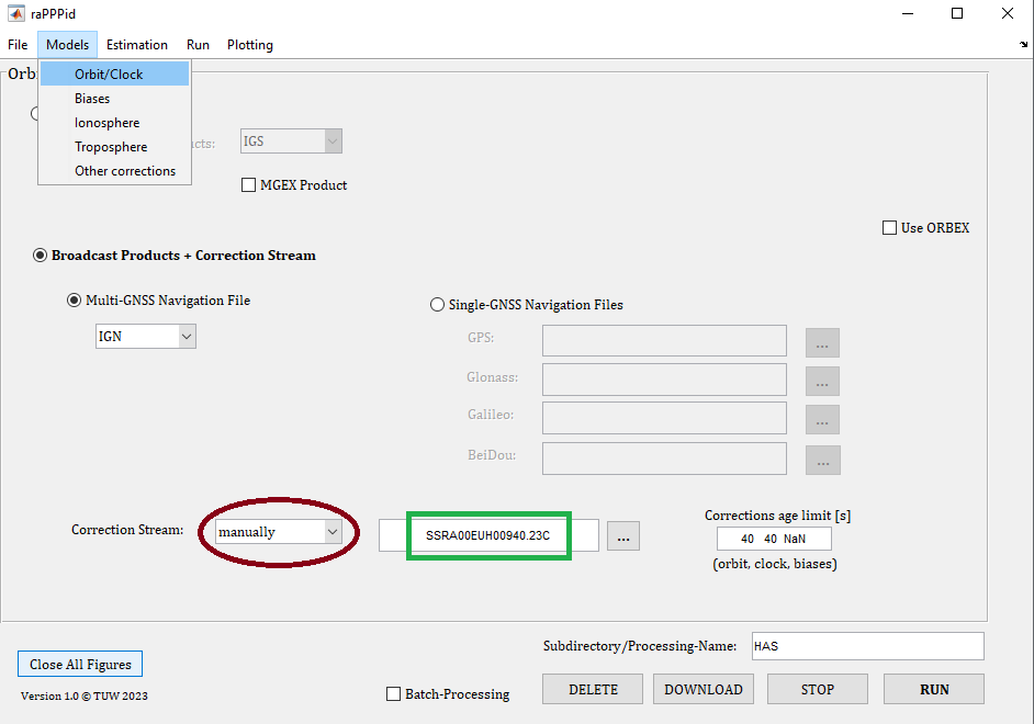
Previously, the corrections from the CNES archive have been used. To apply the correction from the Galileo HAS you have to select the recorded real-time correction stream manually. Furthermore, phase biases have to be deactivated because the Galileo HAS currently does not provide any phase biases. Therefore, change to panel ‘Biases’ (menu item: Models). Set the (Additional) Phase Biases Source to off. Then you can hit the RUN button to start the processing.
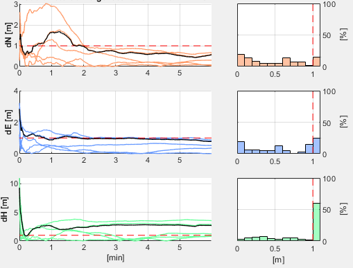
When the processing is finished, change to the Multi-Plot panel. Make sure that all definitions of convergence correspond to one meter, load the reference coordinates of PF04 (check the description above), and try to create the Coordinate Convergence plot. Your plot should look similar to the one provided above.
Congratulations! You have successfully processed raw GNSS data from a smartphone with the Galileo HAS. Although only GPS and Galileo observations are processed sub-meter accuracy is achieved.
Jump to Table of Content