¶ Processing in VieVS VLBI
¶ GUI and batch
A graphical user interface (GUI) for VieVS, 'VIE_SETUP' is provided. All the different modules are integrated in the GUI and can be selected with the drop down menu. Additionally a plotting tool is implemented. The GUI can be started by typing ''vievs'' in the Matlab command window (be sure that the VieVS/WORK directory is set as current directory in Matlab).
¶ Processing preparation done by the GUI
The final purpose of the interface before processing is to save the required files at their required destination. The only difference between the buttons ''Save runp'' and ''Save + Run'' is that the latter also starts the processing (VIE_BATCH). Following files are created when clicking either ''Save runp'' or ''Save + Run'':
- input_protocol.txt - not required for processing
- runp.mat - required in folder /WORK/
- process_list.mat - required in folder /WORK/
- parameter.mat - required in folder /DATA/LEVEL0/subdir/
- Simulation parameters - required for VIE_SIM
- Global parameters - required for VIE_GLOB
¶ Batch processing
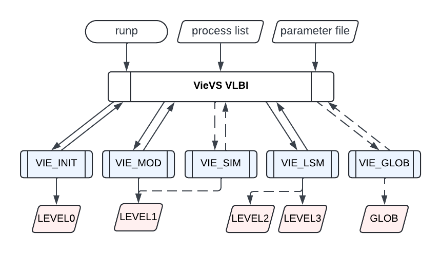
To start the processing, the user has to click either on ''Save + Run'' in the GUI or type ''vievs('batch')'' in the command window (a runp.mat file has to be created beforehand). The chart below shows the workflow of VIE_BATCH, which is called by executing the software. You can see the required input files at the top of the graph and the directories where intermediate and final results are saved at the bottom. In the middle you can see the modules which are used according to the input. Dashed lines indicate optional modules and output. If VIE_SIM is run, the output in the folder LEVEL1 is overwritten and in case a global solution is calculated with the module VIE_GLOB, VIE_LSM saves additional output data in the LEVEL2 folder, which serve as input data for VIE_GLOB.
¶ Parallel computing
To speed up the processing of several sessions with the same parametrization, parallel computing, allows Matlab to use more than one core. Parallel computing can be enabled in Run - run options (see Figure below). The Parallel Computing Toolbox in Matlab is required to run parallel jobs.
When parallel computing is enabled, the sessions run in a parfor instead of a for loop. This decreases the computation time roughly by a factor of the number of cores (usually 2 or 4). If the number of cores in the GUI is set to ''auto'', Matlab uses the number of pools specied by the default parallel configuration.
¶ Estimation
In the tab Estimation, parameters for the estimation process can be selected. The current version supports parameter estimations with the least squares adjustment (LSM). One of our aims is to develop a Kalman Filter as second parameter estimation algorithm. It has not been implemented yet. For the estimation of a global solution the matrix has to be prepared with the LSM module (menu item Global parameters). The corresponding source code can be found in VIE_LSM.
It should be mentioned there that the weighted of the observations are derived by taking the standard deviation of the observations as provided in the NGS files (there are NGS files with different standard deviations available!) plus adding 1 cm quadratically.
¶ Overview of VIE_LSM
The VIE_LSM module was designed by Kamil Teke in the course of his Ph.D. thesis. This section provides a brief discussion of the module and its implementation into VieVS. For further detail see (Teke, 2011).
The VIE_LSM module takes care of the parameter estimation process with the least squares method. All the parameters can be estimated as continuous piece-wise linear offsets (CPWLO) in sub-daily and daily temporal resolution. Pseudo observations (constraints) can be introduced to the estimation process. We distinguish between two types of constraints, namely relative and absolute. Relative constraints are used to fill gaps where two parameters have no observation in an estimation interval. Additionally they provide supplementary observations which keep the normal equation matrix regular. Absolute constraints are used if the preferred value of the parameter is known (e.g. fixing it to the a priori value).
The design matrix is formed by 15 sub-matrices,
The used models are:
- CPWLO of clocks (),
- rate and quadratic terms of polynomials of clocks (),
- CPWLO of zenith wet delay (),
- CPWLO of troposphere north gradients (),
- CPWLO of troposphere east gradients (),
- CPWLO of polar motion coordinates in TRF along the Greenwich meridian () (),
- CPWLO of polar motion coordinates in TRF along east meridian () (),
- CPWLO of Earth's rotation phase (dUT1) (),
- CPWLO of celestial intermediate pole (CIP) coordinate in CRF (X) (),
- CPWLO of celestial intermediate pole (CIP) coordinate in CRF (Y) (),
- CPWLO of right ascensions of source in CRF (),
- CPWLO of declinations of sources in CRF (),
- CPWLO or one offset (optional) of VLBI antenna X coordinate in TRF estimated using all observations (),
- CPWLO or one offset (optional) of VLBI antenna Y coordinate in TRF estimated using all observations (),
- CPWLO or one offset (optional) of VLBI antenna Z coordinate in TRF estimated using all observations (),
- CPWLO of satellite position N/R/X coordinate in the local orbital frame (NTW/RSW/XYZ) (),
- CPWLO of satellite position T/S/Y coordinate in the local orbital frame (NTW/RSW/XYZ) (),
- CPWLO of satellite position W/W/Z coordinate in the local orbital frame (NTW/RSW/XYZ) (),
- CPWLO of semi-major axis of satellite orbit (),
- CPWLO of eccentricity of satellite orbit (),
- CPWLO of inclination of satellite orbit (),
- CPWLO of right ascension of ascending node of satellite orbit (),
- CPWLO of argument of perigee of satellite orbit (),
- CPWLO of argument of latitude of satellite orbit (),
- CPWLO or one offset (optional) of VLBI antenna X coordinate in TRF estimated using satellite observations only (),
- CPWLO or one offset (optional) of VLBI antenna Y coordinate in TRF estimated using satellite observations only (),
- CPWLO or one offset (optional) of VLBI antenna Z coordinate in TRF estimated using satellite observations only (),
- CPWLO or one offset (optional) of VLBI antenna X coordinate in TRF estimated using quasar observations only (),
- CPWLO or one offset (optional) of VLBI antenna Y coordinate in TRF estimated using quasar observations only (),
- CPWLO or one offset (optional) of VLBI antenna Z coordinate in TRF estimated using quasar observations only ().
¶ Troposphere
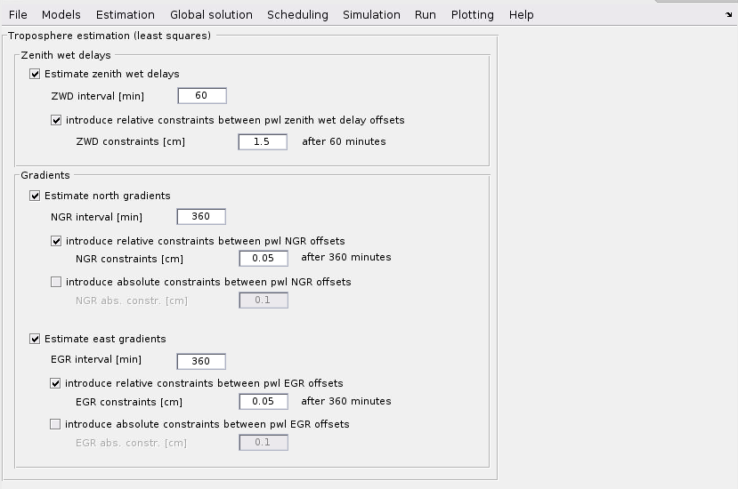
The estimation settings for the troposphere can be found in Estimation - Least squares - Troposphere a screen shot of the GUI is depicted in Figure below. We usually estimate the zenith wet delay and north and east gradients. Both are estimated as CPWLO, intervals and constraints can be selected in the GUI. If nothing is changed the predefined default values are used.
¶ Clock
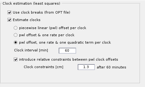
Estimation settings for clock parameters can be found in Estimation - Least squares - Clock A screen shot of the GUI is depicted in the Figure below. One can specify if clock breaks from an OPT file should be used.
In order to estimate clock errors a reference clock has to be selected. The clock of the first station in the _antenna.mat file is chosen as default. One can specify any other clock as reference in the OPT file. The deviation of the other clocks w. r. t. the reference clock is then modeled according to the selection of the user. The CPWLO for each clock at each UTC integer hour or any other user defined interval ( and ) is modeled according to:
and the quadratic polynomial term is estimated with:
The total clock error at the epoch is the summation of the CPWLO for each clock and the quadratic polynomial term for each clock:
Relative constraints can be introduced by the user.
¶ Earth orientation parameters
The settings of the EOP estimation can be changed in Estimation - Least squares - EOP. A screen shot of the GUI is depicted in Figure below. It is possible to estimate EOP (with the CPWLO method) in any given interval with specified constraints. One can fix the EOP to the a priori values by ticking off the parameters respectively.

¶ Station coordinates
The settings for station coordinate estimation can be found in Estimation - Least squares - Station coordinates.
To specify the datum of the network one has to define the origin and orientation of the coordinate system. This can either be done by fixing station coordinates to their a priori (TRF) values or by introducing the no-net-translation (NNT) and no-net-rotation (NNR) conditions. To fulfill the NNT condition the three translations are constrained to zero. The NNR condition is fulfilled when all three rotations are constraint to zero. The standard approach for VLBI estimation typically involves applying No-Net-Rotation (NNR) and No-Net-Translation (NNT) constraints when a session includes only observations to geodetic (quasar) sources. However, if the session contains both quasar and satellite observations, users can decide which types of observations are used for the station coordinate estimation.
Station coordinates can be estimated in several ways:
- using all observations (quasars and satellites),
- using only satellite observations,
- using only quasar observations, or
- estimating two separate sets of station coordinates simultaneously — one from quasar observations and one from satellite observations.
In the last case, the user can choose which of the two solutions is written to the SINEX file. For that case, the NNT condition is applied only to the station coordinates derived from quasar observations and no NNT constraint is applied to the station coordinates estimated from satellite observations.
The no-net-scale (NNS) condition (constraining the scale to 1) is usually not used for VLBI parameter estimation.
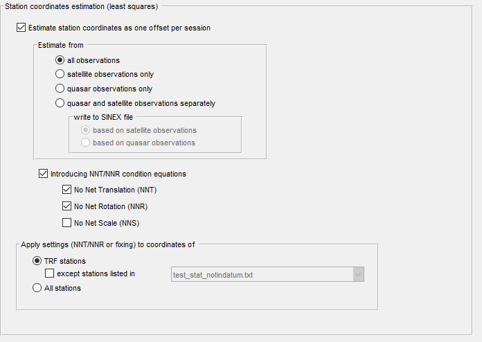
Coordinates are estimated daily. The Estimation of sub-daily antenna TRF CPWLO coordinates with NNR/NNT conditions is not yet implements in VIE_LSM.
¶ Source coordinates
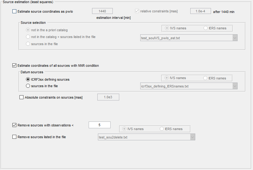
VieVS is able to estimate source coordinates. The settings can be found in Estimation - Least squares - Source coordinates. Source coordinates can be estimated as pwl offsets (estimation interval and relative constraints are selected in the GUI), or with NNR condition. If you ticked the pwl offset estimation, it can be chosen which sources are to be estimated. The NNR option estimates all sources with a loose constraint (can be specified in the GUI) applied on all sources. In the NNR condition only sources in the chosen catalogue are included by default, if not specified otherwise by using selected sources listed in the .txt file. It is possible to remove sources which are observed less than five times or specific sources listed in a .txt. file. By default the NNR is selected for the estimation of source coordinates.
From Version 3.0 sources observed less than 3 times are automatically excluded from the NNR condition, or in case the pwl offset estimation is applied they are fixed to their a priori coordinates.
¶ Satellite Position
If observations to satellites are included in the session, their positions can be estimated. In Estimation - Least squares - Satellite position specifications can be made.
Users can select:
- the reference frame in which the satellite positions are estimated, and
- the time interval (in minutes) for the piecewise-linear (PWL) satellite position estimation.
The available reference frames include:
- NTW (Normal, Tangential, Cross-track),
- RSW (Radial, Along-track, Cross-track),
- TRF (Terrestrial Reference Frame), and
- GCRF (Geocentric Celestial Reference Frame).
Additionaly, relative constraints can be applied in order to avoid large differences in the satellite position offsets between two consecutive PWL satellite positions.
The radial or normal component of the satellite position can be constrained to its a priori value. A weighting factor can be applied to control the strength of this constraint.

¶ Orbital Elements
In case a session contains observations to satellites, their orbital elements can be estimated within the session analysis. If this should be done, the checkbox Estimate Orbital Elements in Estimation - Least squares - Orbital Elements must be checked.
Once activated, the method for computing the partial derivatives of the time delay with respect to the orbital elements can be selected.
The available options are:
- numerical derivatives based on the time delay
- numerical derivatives based on the satellite position,
- analytical derivatives
At the bottom of the interface, users can select which orbital elements should be estimated, as well as define the time interval over which the estimation is performed.

¶ Weight matrix!
Default settings
Weight matrix of observations is a diagonal matrix. The main diagonal contains 1/m_ni^2, where m_ni^2 is a sum between the squared formal error reported by the correlator (stored in the NGS file) and squared one centimeter error (33ps) for each observation.
There is a possibility to down-weight certain stations in the OPT file.
Baseline dependent weights
Another option is to use the baseline dependent weights. The least square adjustment is run iteratively in two steps. In the first run the vector with residuals for each observation is obtained (using the default settings), in the second run the new matrix is created where the mean value over same baselines is added. You can choose this option in GUI Run - VieVS estimation settings under "Apply baseline dependent weights". The creation of the baseline dependent matrix was coded by Minttu Uunila.
Elevation dependent noise
When choosing the elevation dependent noise, terms dependent on the elevation of the antennas for the respective observation are added to the squared formal error reported by the correlator, instead of the squared one centimeter error:
You can choose this option in GUI Run - VieVS estimation settings under "Introduce elevation dependent noise".
¶ Global parameter estimation
¶ Introduction
Module Vie_GLOB has been designed and written by Hana Krásná in connection to her Ph.D. thesis. It has the capability to estimate parameters which are common to all VLBI sessions from a so-called global solution, i.e. from a common adjustment of many VLBI sessions. The input data for Vie_GLOB are datum-free normal equations (NEQ) prepared by the module Vie_LSM. The global solution is typically used to determine TRF in terms of station positions and velocities, and the CRF in terms of radio source coordinates.
¶ Estimated parameters (Version 3.0)
¶ Parameters estimated from combination of more sessions
- station coordinates and velocities: TRF
- source coordinates: CRF
- Earth orientation parameters
- antenna axis offset
- station seasonal harmonic signal (annual + semi-annual period)
- tidal ERP variations
- pole tide Love/Shida number
- APL regression coefficients
¶ Session-wise reduced parameters
- zenith wet delay
- tropospheric gradients
- Earth orientation parameters
- station and source coordinates (not suitable for global estimation)
¶ Input data
For each session there are 3 files: (* denotes name of the session, i.e. 10JAN04XA_N004)
- *_an_glob.mat (in Vie_GLOB the name of this matlab structure is glob1)a priori station coordinates and velocities used for analysis in this session + information about discontinuities
- *_Nb_glob.mat (glob3) datum free normal matrix and right-hand side vector
- *_par_glob.mat (glob2) glob2.x - information about columns, where the parameters are stored. It also contains estimates from the single session adjustment with Vie_LSM. glob2.opt - information about options, which were chosen for the analysis with VieVS and for preparation of the LEVEL2 data.
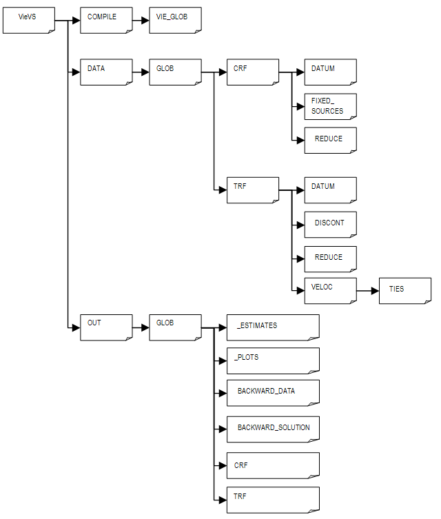
Description of the external files needed for Vie\GLOB (VDG = VieVS/DATA/GLOB):
| Directory | Description |
|---|---|
| VDG/CRF/DATUM/ | arbitraryname.txt files with source names, which will be used for an NNR condition |
| VDG/CRF/FIXED_SOURCES/ | arbitraryname.txt files with source names, which will be fixed to their a priori coordinates (i.e. they will be not involved in the adjustment) |
| VDG/CRF/REDUCE/ | arbitraryname.txt files with source names, which position will be session-wise reduced |
| VDG/TRF/AO/ | arbitraryname.txt files with station names, where the axis offset will be estimated |
| VDG/TRF/APLRG/ | arbitraryname.txt files with station names, where the APL regression coefficients will be estimated |
| VDG/TRF/DATUM/ | arbitraryname.txt files with station names, which will be used for an NNT/NNR condition |
| VDG/TRF/DISCONT/ | arbitraryname.mat files with station names describing the VLBI position discontinuities. The original VLBI-DISCONT.txt file is provided at the web site http://vlbi.geod.uni-bonn.de/IVS-AC/data/VLBI-DISCONT.txt (vlbi\discont.mat is provided within vie\glob and at least one file must be in the ../DISCONT/ directory (also if station coordinates are not estimated)) |
| VDG/TRF/REDUCE/ | arbitraryname.txt files with station names, which position will be session-wise reduced. Their velocity will be fixed to the a priori value |
| VDG/TRF/STSEASON/ | arbitraryname.txt files with station names, where the seasonal harmonic signal (annual + semi-annual period) will be estimated |
| VDG/TRF/VELOC/ | arbitraryname.txt files with station names, at which a position discontinuity happened, but we want to estimate a constant velocity for all intervals |
| VDG/TRF/VELOC/TIES/ | arbitraryname.txt files with station names in a special format: names of antennas (8 character for each), the line has to end with "\textbackslash". Velocity ties will be introduced to stations at one line and the same velocity will be estimated for them. |
| VieVS/OUT/GLOB/*.m | Matlab function backward\solution.m estimates after the global adjustment the session-wise reduced parameters. The plot\backward*.m functions plot the time series of the session-wise estimated parameters (= output of backward\solution.m) |
| VieVS/OUT/GLOB/ | directories / mat. files are for outputs - data will be automatically written into them |
Structure of Vie_GLOB in the VieVS directories:
¶ Program
The computational strategy of Vie_GLOB follows several steps. First, information from all sessions is read to detect all parameters which are contained in the input normal equations. Only parameters of interest for the global solution are kept in the session-wise NEQ and the remaining parameters are either fixed to their a priori values or reduced from the equations. This can be specified in the GUI, see Figure:
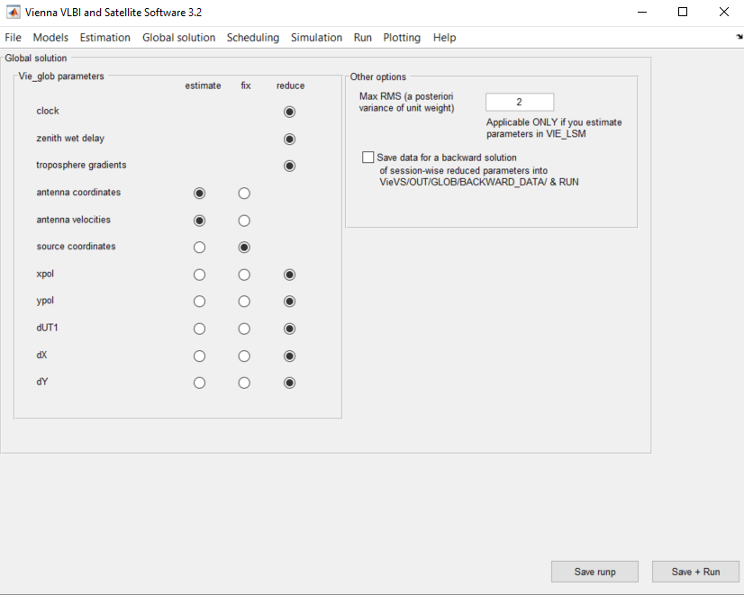
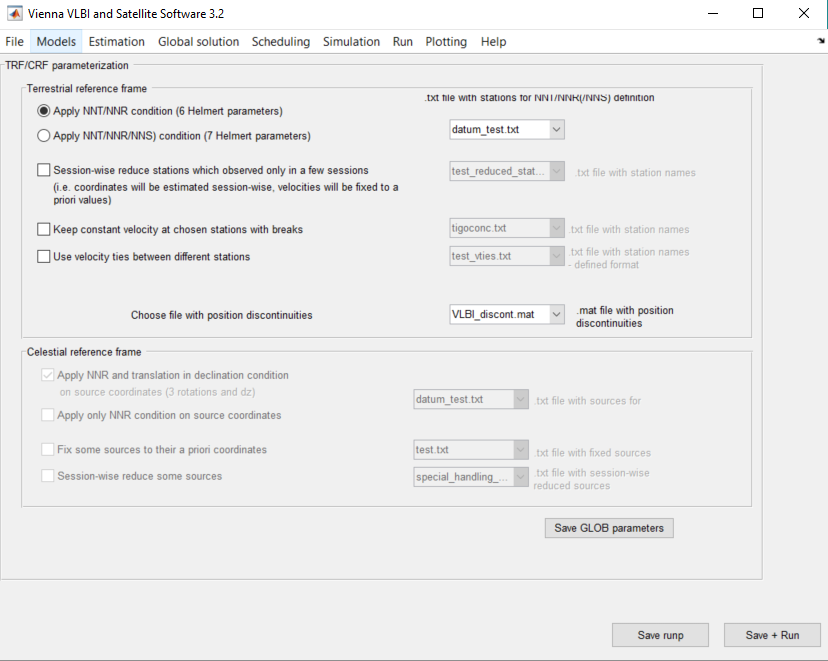
The reduction takes place for parameters which appear in one session only and are dependent on a finite amount of time. These are, for example, the clock parameters, zenith wet delays or tropospheric gradients which can vary by several hours. The reduction means an implicit estimation of such parameters from the session-wise NEQ by a least squares adjustment. The global parameters are detected in the NEQ taken from single sessions, and a new reference number is assigned to each parameter. In the second step of Vie_GLOB the NEQ are reorganized following the new order of parameters (columns/rows in normal matrix and rows in normal vector) and stacked together with the reorganized NEQ from other sessions. This leads to one common global normal matrix which consists of the global parameters only. In the third step conditions (like no-net-rotation and no-net-translation on TRF or no-net-rotation on CRF) and eventually constraints are applied (see Figure below for GUI settings), and by a final inversion of the NEQ system the estimates of the global parameters are obtained. In a usual run of Vie_GLOB where we are only interested in the global parameters (e.g. in a new reference frame) the analysis stops at this stage. However, if we are also interested in the solution for parameters which have been session-wise reduced, a backward solution has to be carried out. This means that the residuals estimated for the global parameters are taken and substituted into the reduced equation going step by step always one level up.
¶ Reduction and stacking of parameters
The reduction of parameters is based on a division of the normal equation system into two parts. In the first part those parameters are concentrated, which will be kept in the global matrix, and in the second part parameters are ordered, which will be estimated only from a single session:
The matrix equation above corresponds to the following two coupled equations:
From the equation above vector can be expressed containing the reduced parameters:
and substituted into the equation for :
The reduced N matrix and the reduced b vector are than "stacked" with reduced normal equation systems from other sessions and a global N matrix and a global b vector is created. Attention has to be paid so that the order of parameters is identical in the reduced normal equation systems:
The final solution for the global parameters is done using an inversion of the global normal equation system:
The estimates of the session-wise reduced parameters can be obtained by substituting the vector into the equation for , where and thus contains the globally adjusted parameters. It is obvious that one has to store the matrices , and vectors of each session. To obtain the time series of the reduced parameters from all sessions it should be started with the reduced normal
¶ Output data
¶ Output figures
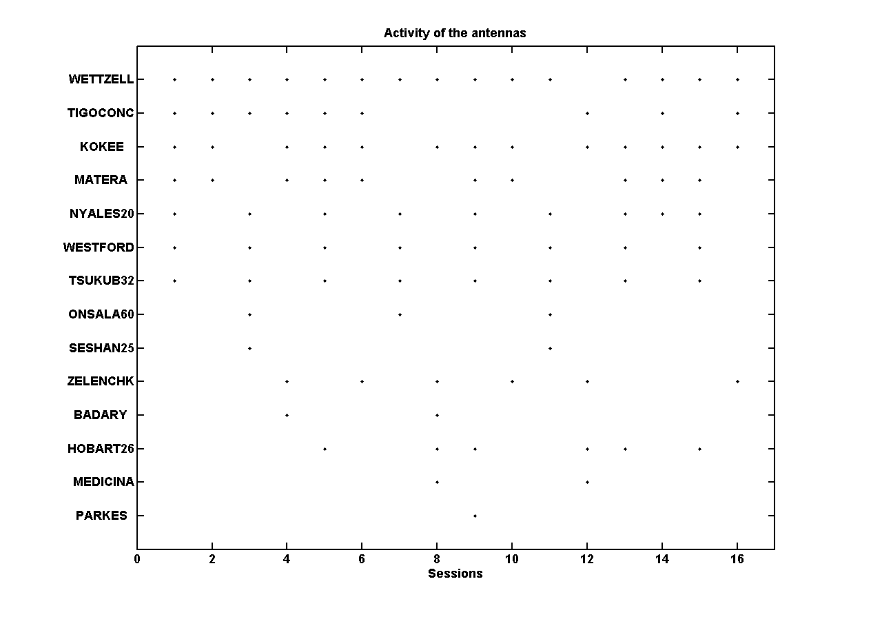
Output figures are saved in VieVS/OUT/GLOB/_PLOTS/TEST_OUT (source code for saving the figures is at the very end of the main program Vie_GLOB.m). The figure below shows stations in sessions included in the global adjustment. It is created with the function plot_antactiv.m. It is stored in VieVS/OUT/GLOB/_PLOTS/TEST_OUT/ant_activity_TEST_LEVEL2.eps.
The figure below shows the map with all stations included in the global adjustment. Blue circles denote stations included in the NNT/NNR condition, red circles show stations excluded from the NNT/NNR condition. It is created with the function plot_ant.m. It is stored in VieVS/OUT/GLOB/_PLOTS/TEST_OUT/ant_map_TEST_LEVEL2.eps.
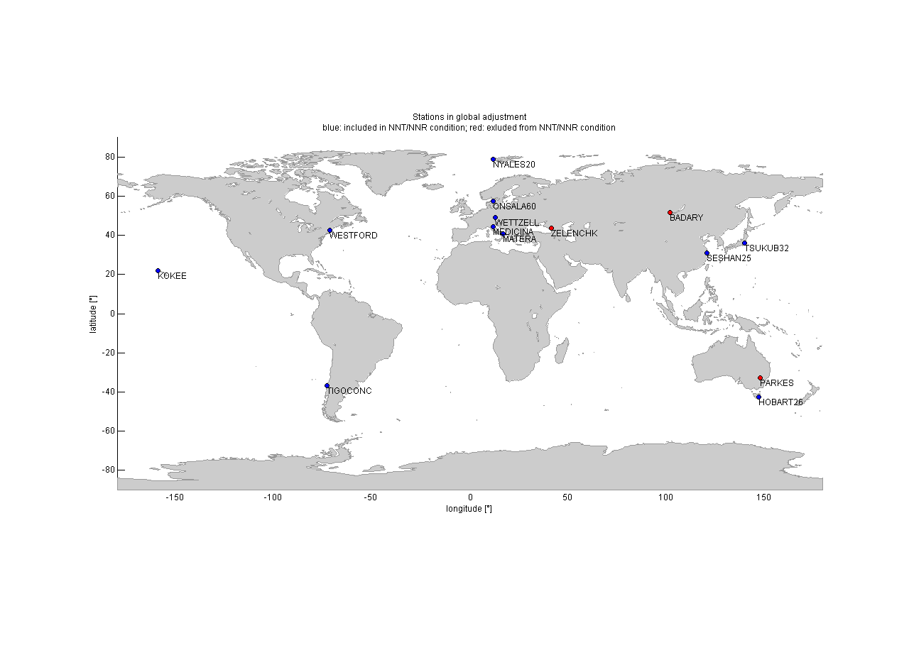
The figure below shows the map with all stations included in the global adjustment. Blue circles denote stations included in the NNT/NNR condition, red circles show stations excluded from the NNT/NNR condition. It is created with the function plot_ant.m. It is stored in VieVS/OUT/GLOB/_PLOTS/TEST_OUT/ant_map_TEST_LEVEL2.eps:
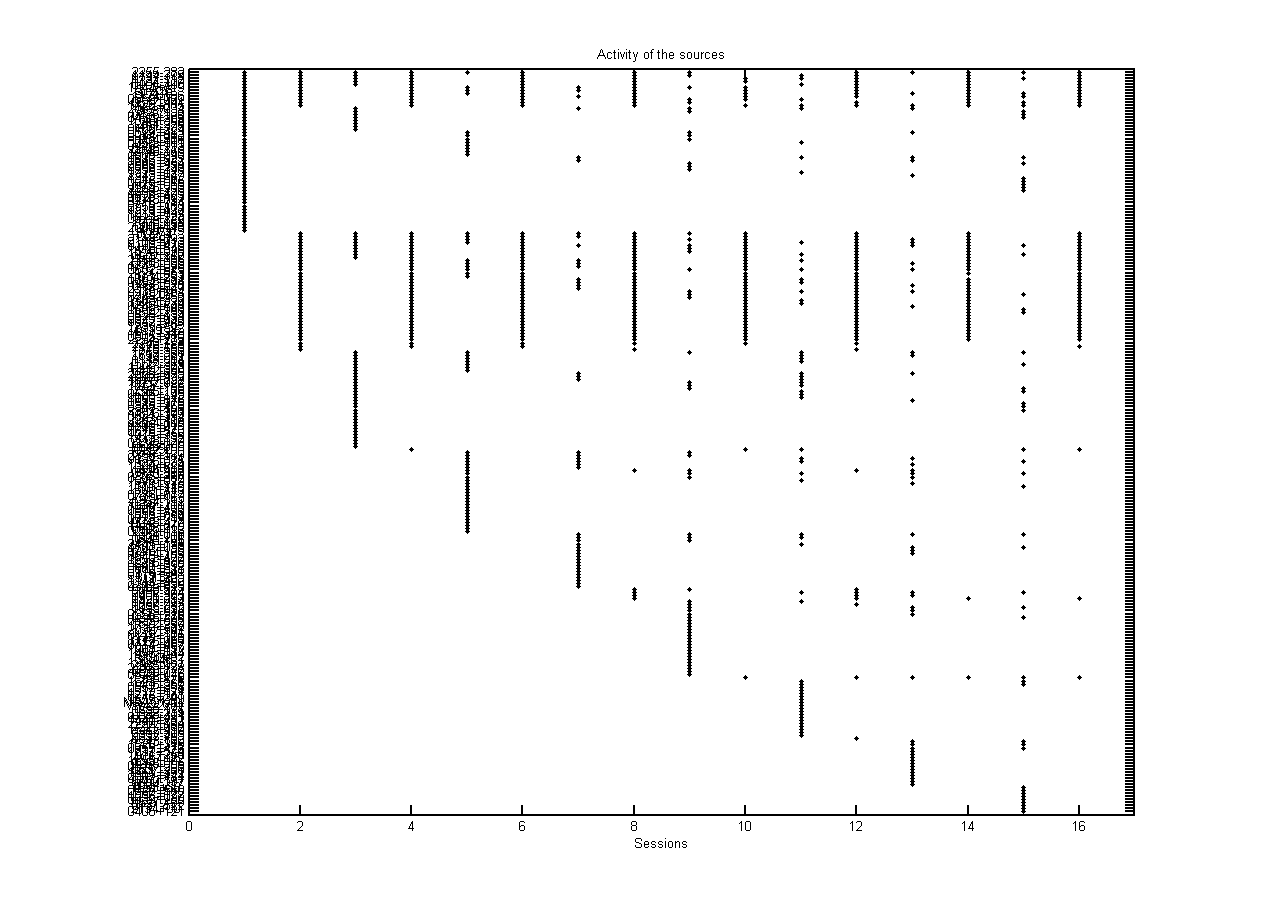
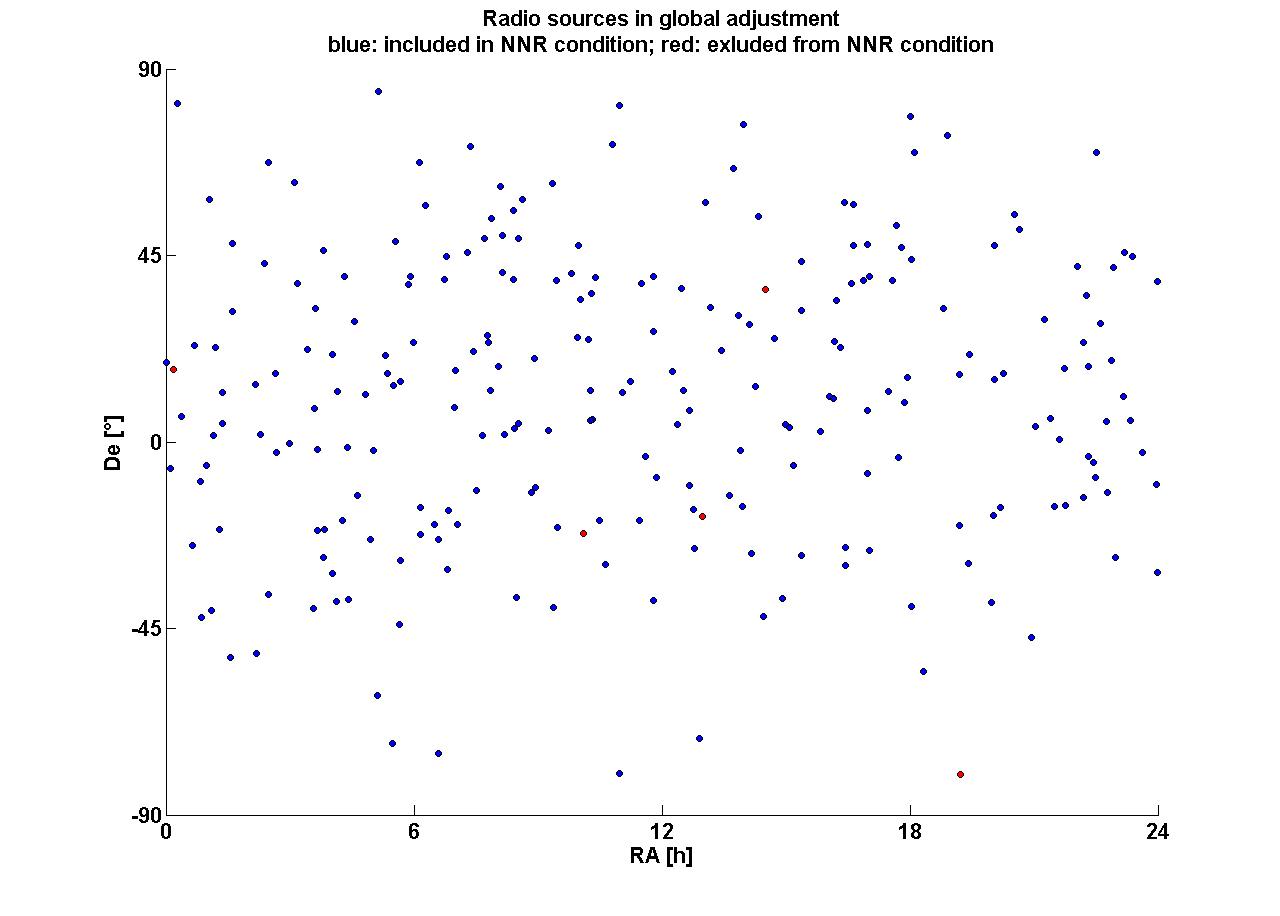
Thew figure below shows the map with all sources included in the global adjustment. Blue circles denote sources included in the NNR condition, red circles are sources excluded from the NNR condition. Sources which were fixed to their a priori coordinates are not shown. It is created with the function plot_sou.m. It is stored in VieVS/OUT/GLOB/_PLOTS/TEST_OUT/sou_map_TEST_LEVEL2.eps:
¶ Results
Estimates are stored in VieVS/OUT/GLOB/_ESTIMATES/TEST_OUT/:
- in Matlab format: globsol_TEST_LEVEL2.mat
- in TXT format: glob_results_TEST_LEVEL2.txt
¶ global EOP
You can use vie_glob to estimate EOP. The advantage is, that instead of the usually 3 values for the single session solution, the EOP series of the consecutive sessions are combined. This gives you one value per day. Important: if you want to globally estimate EOP, choose loose constraints (e.g. 1 mas) in the single session solution.
¶ Simulation
¶ Overview of VIE_SIM
With the VieVS simulation module (VIE_SIM) simulated VLBI observables are generated, taking into account the three most important stochastic error sources in VLBI (additionally the simulation of source structure was added later on). VIE_SIM sets up the o-c vector (observed minus computed) of the least-squares adjustment at each epoch. The artificial observations from the VieVS simulator (VIE_SIM) are then transformed to databases in NGS format.
Group delay observables are calculated containing the following four main stochastic error sources in VLBI: The wet troposphere delay, the station clock error, the measurement noise and the source structure (see Equation below). The wet troposphere delay has the largest impact on the error.
and are the simulated zenith wet delays and clock values at the station 1 and 2 and are the corresponding wet mapping functions for the elevation angles which are assumed to be error-free. The source structure () and the white noise () are added per baseline.
¶ Input files
¶ NGS or vgosDB
You can select the sessions to be simulated in the GUI (File - Set input files), e.g. from the VieVS/DATA/NGS if you are selecting 'Browse for sessions' or from the VieVS/DATA/vgosDB folder when selecting 'Browse for VGOSDB'.
¶ Simulation parameters
Some input simulation parameters files are located in the /VieVS/DATA/TURB/ folder. They contain station names (8 characters), the refractive index structure constant [], the effective height of wet troposphere [m], components of the wind vector [m/s], the a priori zenith wet delay [mm], the correlation interval [m], the step width for the numerical integration [m], the clock Allan Standard Deviation and the white noise [ps].
However, it is possible to select the simulation parameters in the GUI in the Simulation section. Furthermore, the selected parameters can be saved as a .mat file to be used in further processing/ simulations.
¶ Output files
The simulated NGS files are stored in the DATA/SIM/your_dir/year directory. In DATA/LEVEL4 you find a Matlab structure file with the simulation parameters used in the processing.
Additionally, if vie_lsm is executed, parameters like the mean formal error and the repeatabilities of the estimated parameters can be found in VLBI/OUT/your_dir.mat.
¶ Perform simulations
After starting Matlab you should select the VieVS/WORK/ directory as current folder. Typing "VieVS" in the Matlab command window starts the interface of the latest version of VieVS.
- In the GUI (File - Set input files) you can choose the sessions to be simulated. Do not use outlier files and, if OPT files exist, create an empty OPT directory (e.g. 'SIM'). Select this directory in the GUI before starting the simulator.
- In the GUI (Parameters - observation restrictions) set the quality code limit to a large number ().
- After you select the Simulation menu label on the top of the interface, the interface of VIE_SIM appears (as shown in the Figure below). You can choose the parameters to be simulated and enter the number of days and a starting point for the running number of the NGS files. The additional options include 'set reference clock to zero' and 'write ngs file'. You can choose a file containing the simulation parameters (stored in VieVS/DATA/TURB/ folder). An alternative option is to directly enter the values, these will then be applied to all stations. If you want to simulate source structure as well you have to select a predefined catalog which contains the source structure of every source. It shall be noted here, that while clk, trp and wn have a stochastic component that changes for each simulation run, source structure is a geometrical quantity and is identical for the individual observations in repeated simulation runs. Hence it is a systematic effect.
- In the menu (Run - Run options) the checkboxes VIE_INIT, VIE_MOD and VIE_SIM have to be selected to run the simulation.
- It is possible to do the simulation and parameter estimation in the same run. Just add the checkbox VIE_LSM.
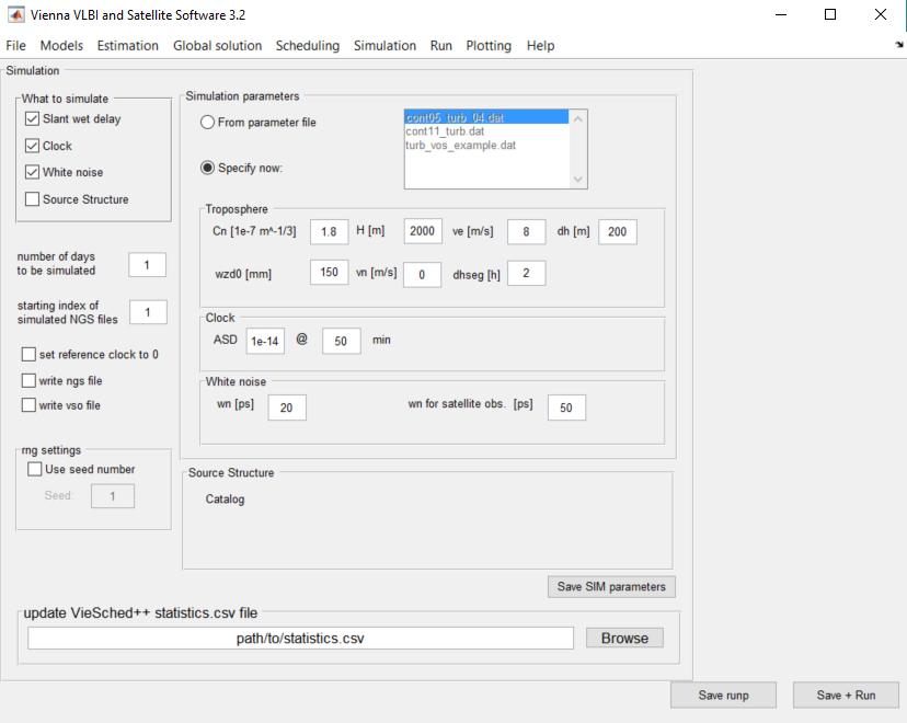
The simulation tool is very useful to test different schedules. Make sure to create an NGS file while running VIE_SCHED and use this file to do the simulations. You can even do everything at once by selecting all the modules (VIE_SCHED, VIE_INIT, VIE_MOD, VIE_SIM, VIE_LSM) in the Run - Run options menu.
¶ Running VieVS VLBI
¶ Sinex output
The SINEX file format is a standardized output ASCII format used by the International Earth Rotation and Reference Systemsn Service (IERS). It is used for the distribution of products and estimates. VieVS is capable of writing SINEX files as output. This option is given in Run - Sinex output. Only values which are estimated can be chosen. The option 'include' writes the chosen parameters to the SINEX files. Zenith wet delays are usually estimated every hour. Therefore the normal equation matrix (and also the SINEX file) would become very large. The option 'reduce from N matrix', removes the entries for the chosen parameters (e.g. zenith wet delays) from the normal equation matrix and makes the SINEX files considerably smaller. However, the parameters can be derived from the 'reduced' N matrix as well.
¶ VieVS estimation settings
In the VieVS processing settings (Run - VieVS processing settings) the user can select the clock parametrization in the first solution (in which only one zenith wet delay per station and one linear clock function per station is estimated) and the outlier test in the main solution (in which all parameters are estimated). Furthermore the user can (de-)select to actually estimate parameters (otherwise only the normal equation matrix is set up) and start a station- and source wise parametrization for each session chosen in File - Set input files.
There is a button to save a current parametrization to an ASCII file in this panel as well.
¶ Run options
In Run - Run options the user can basically chose which modules should be run and to which subfolders the (intermediate) results should be saved to. The results are saved in the VieVS/DATA/LEVELx/ subfolder/.
In the "Advanced options" section the user can specify if he wants to run the process_list in parallel.
Another option worth mentioning is the exception handling which can be specified in here. If you deselect the "stop process list if there is an error in a session" checkbox VieVS will not stop when an error is found in a session. The error will be printed on the screen and the next session in line will be started. When VieVS is finished all failed sessions are printed in the commandwindow. Furthermore, a process list with all the failed sessions is saved at WORK/PROCESSLIST/failed_sessions.mat. This list can then be used for investigating the errors. The exception handling also works in parallel mode. This option is particularly usefull when large process lists are used, because it can run unattended and failed sessions can be looked at alltogether after the process list is finished.