¶ Residuals
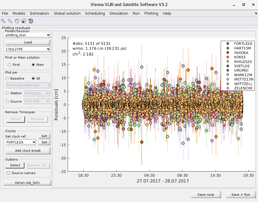
The residual plotting tool is shown in the Figure below. It allows the user to plot residuals from first (only clock functions and one zenith wet delay per station estimated) and main (all parameters estimated) solutions. Those can furthermore be visualized per station, per baseline and per source to e.g. detect problematic sources, stations or baselines.

By clicking Load all sessions in the chosen folder ('/' corresponds to /DATA/LEVEL3/ are loaded by the program and shown in the second popupmenu. In the second popupmenu you can switch to a particular session, which will be displayed in the window immediately. If nothing seems to happen the chosen folder might be empty.
- Note, that the res_ files are loaded only.
- Hint, the outliers will be highlighted by black crosses, only if in Run→VieVS estimation settings in box: Main solution (box is checked) you were chosen whether the simple or normal outlier test and processed the data with this parametrization.
¶ Adding clock break information
If a session contains a clock break, a jump in the residuals at the epoch of the clock break might be observed. This can be removed interactively when station-wise residuals are plotted. The user has to click Add clock break, select the time epoch of the clock break (simply click with the white cross on the plot; the y-value is not important) and confirm that the information is written to the OPT-file. The OPT-folder will be the same as chosen in File - Set input files. The clock-break will be applied the next time this session is analyzed with VieVS.
¶ Removing outliers manually
Outliers can be removed by clicking Select outliers in the residual plot window. The user can either click on one value or drag-open a box containing the outlier values. All values will be marked with black crosses. To write all those values to the OUTLIER file, the button Remove Outliers must be pushed. Similar to the clock break information, the outlier information is written to the outlier folder selected in File - Set input files. The outliers will be removed right at the beginning in all following VieVS runs.
¶ Residual plot features
In this block you can select data on the residual plot manually or you can assign a particular time span during session time. The selected data are written in the OPT-file.
It is designed to do the selection as follows:
- Click on Select . Now, Select Data is active.
- You can start working with whether First or Main solution, it is also applicable for All, Baseline, Station and Source in block of Plot per. However, you can remove data only per Station and Source, so that button Remove and corresponded action is not available in other positions Plot per .
- End this activity by clicking on Select once more. If you switch cursor in the other boxes or push any button this acting will be finished automatically.
Select time span by your mouse on the window. As a result of your action you will see the vertical lines, which you can change.
¶ Data removing
The selected data for Station or Source in the block Plot per can be removed by writing in OPT-file. Whatever time span you selected, click on Remove. An appeared info message lists the time span which you are going to write down in OPT-file and the directory where this file is located. You can confirm this action YES or cancel NO.
- Reminder, the path for OPT-file is assigned in menu File → Set input file → OPT file.
- Hint, you can remove whole data for station or source by choosing time span limits bigger than observations were done.
- Note, whatever units you selected, time span will be written down to OPT-file in MJD.
¶ Parameters
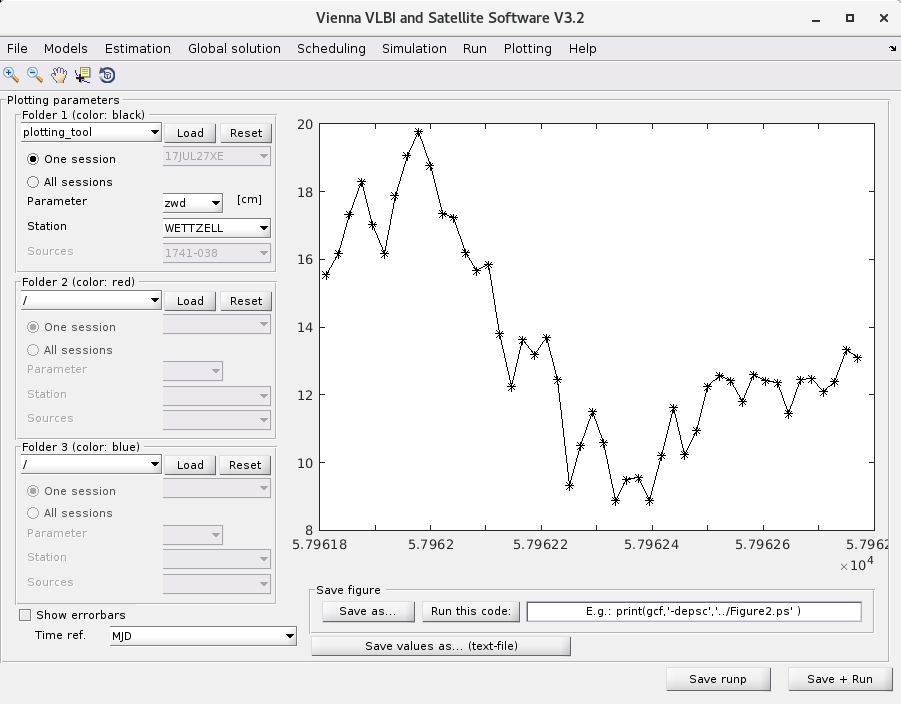
To visualize estimated parameters, VieVS includes a plotting window (Plotting - parameters. Besides the axes on the right, there are three panels where you can load data separately - the three panels plot the data in different colors (panel1: black, panel2: red, panel3: blue) for e.g. comparison. To load data, select the subfolder you chose before processing (if you did not select any, leave '/') and click on Load. All the sessions which are in the selected directory appear in the popupmenu One session. Select this radiobutton to plot single session, otherwise (if you want to plot parameters from all those sessions) click All sessions. Select the parameter and station (only needed for station dependent parameters, such as station coordinates, zenith wet delays or tropospheric gradients) and select Plot below. If nothing appears on the axes, the parameter you selected was not estimated for the chosen session.

- Hint, to make box next to the radio button One session active, switch to All sessions and return to One session. A data for a selected single session will be appeared immediatelly, if x_ includes them.
- Units for chosen parameter is mentioned in the brackets like [cm] for zwd.
- Also you can remove data from the plot by clicking Reset. Note, that you can still access them without loading the folder again: switch the radio button between All sessions and One session.
You can save values depicted in the window to the text file by clicking Save values as … (text-file) or as a figure-file Save as … below.
- Hint, all shown in the window data will be saved in the text or figure file. If you would like to save the data of the particular directory, click Reset to remove data of the other folders.
¶ Session analysis
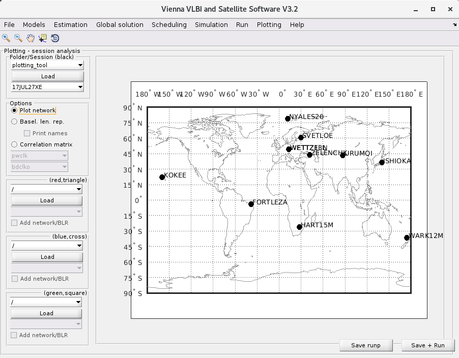
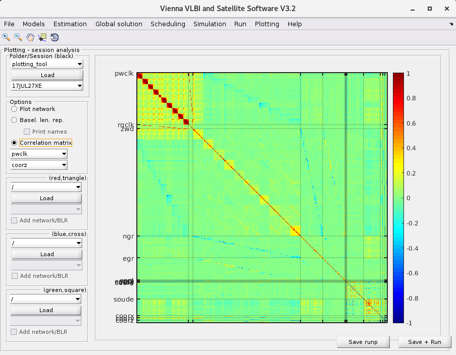
In Plotting - Session analysis next session-related informations can be plotted:
- The station network of one session on the global map;
- The baseline length repeatability based on all sessions in the chosen folder (standard deviations of baselines from all sessions in the chosen folder);
- The correlation matrix of the chosen session. It is available for the sessions in the Folder/Session (black) only.
- Note, that data for the Folder/Session (black) will be plotted in any case.
Up to four sessions can be selected to visualize the station network. The baseline length repeatability can be plotted for up to four data sets (do not forget to check Add network/BLR below the folder).
- In each of four boxes chose the folder and push Load;
- Click Add network/BLR to add corresponded data in the window;
- In each of four boxes you can select one session to plot the station network in the window.

